
🎧 Listen to the Download
Hey data explorers, I’m diving into the latest Download, and let’s be honest: in the world of data, size matters—and so does speed. You wouldn’t bring a butter knife to a sword fight, so why are you trying to wrangle multi-million row datasets with tools that just aren’t up to the task? This issue gives us the essential playbook. We’re getting a clear-eyed look at which analytical engines deliver the goods—DuckDB, I’m looking at you 👀—and, more importantly, we’re settling the age-old ETL debate: Static vs. Dynamic SQL. If your current data pipeline feels less like a well-oiled machine and more like a series of awkward manual updates, you need this. Time to get off the maintenance merry-go-round and build something that can actually scale. Let’s see how you can move your infrastructure from “fine for now” to “production-grade powerhouse.”
Checkout Synoposis, the LinkedIn newsletter where I write about the latest trends and insights for data domain. Download is the detailed version of content covered in Synopsis.
Data‑Bite: Speed‑Showdown of DuckDB, SQLite, and Pandas
Came across an interesting benchmark comparing DuckDB, SQLite, and Pandas on a 1M+ row dataset. The analysis focused on execution time and memory usage across four common analytical queries. Here’s a quick summary of the methodology and findings:
1. Environment and Tool Setup
The primary goal was to ensure a fair testing environment by running all tools within the same Jupyter Notebook.
Software Installation: Installed and imported necessary Python packages: pandas, duckdb, sqlite3, time (for execution time), and memory_profiler (for memory usage).
Data Preparation: The Bank dataset from Kaggle (over 1 million rows) was used.
The data was initially loaded into a Pandas DataFrame (df = pd.read_excel(...)).
2. Data Registration and In-Memory Setup
The loaded Pandas DataFrame was made accessible to all three tools, ensuring they operated on the identical dataset in memory.
Pandas: Queried the DataFrame (df) directly.
DuckDB: The DataFrame was registered directly as a DuckDB table (duckdb.register("bank_data", df)), allowing SQL queries against it without explicit data conversion.
SQLite: The DataFrame was copied into an in-memory SQLite database connection (conn_sqlite = sqlite3.connect(":memory:")) and saved as a table (df.to_sql("bank_data", ...)).
3. Benchmarking Methodology
The comparison focused on four common analytical tasks that mirror real-world data analysis, using the same in-memory data setup for each engine.
A. Consistent Query Execution The same four queries were executed on DuckDB (via SQL on the registered DataFrame), SQLite (via SQL on the in-memory database), and Pandas (via native DataFrame methods).
B. Performance Metrics Measurement Execution Time (Speed): Measured using Python’s time module. The start/end timer was wrapped around the query execution only, excluding data loading and preparation.
Memory Usage (Efficiency): Estimated by sampling memory usage immediately before and after each query using memory_profiler, capturing the incremental RAM consumption in megabytes (MB).
C. The Four Benchmark Queries (Analytical Tasks)
- Total transaction value: Simple aggregation (SUM) of a numeric column.
- Group by domain: Aggregation (SUM) of transaction counts grouped by a single categorical field.
- Filter by location: Filtering rows by a condition (Location = ‘Goa’) before aggregation (SUM).
- Group by domain & location: Multi-field aggregation (AVG) grouped by two categorical fields.
4. Results Analysis and Visualization
The measured execution time and memory usage for all queries and tools were collected, stored, and then compared.
Data Collection: Results (engine, query, time, memory) were compiled into lists of dictionaries, which were then converted into Pandas DataFrames for analysis.
Visualization: Bar charts were generated using matplotlib for a visual comparison of Execution Time (seconds) and Memory Usage (MB) for each query and tool.
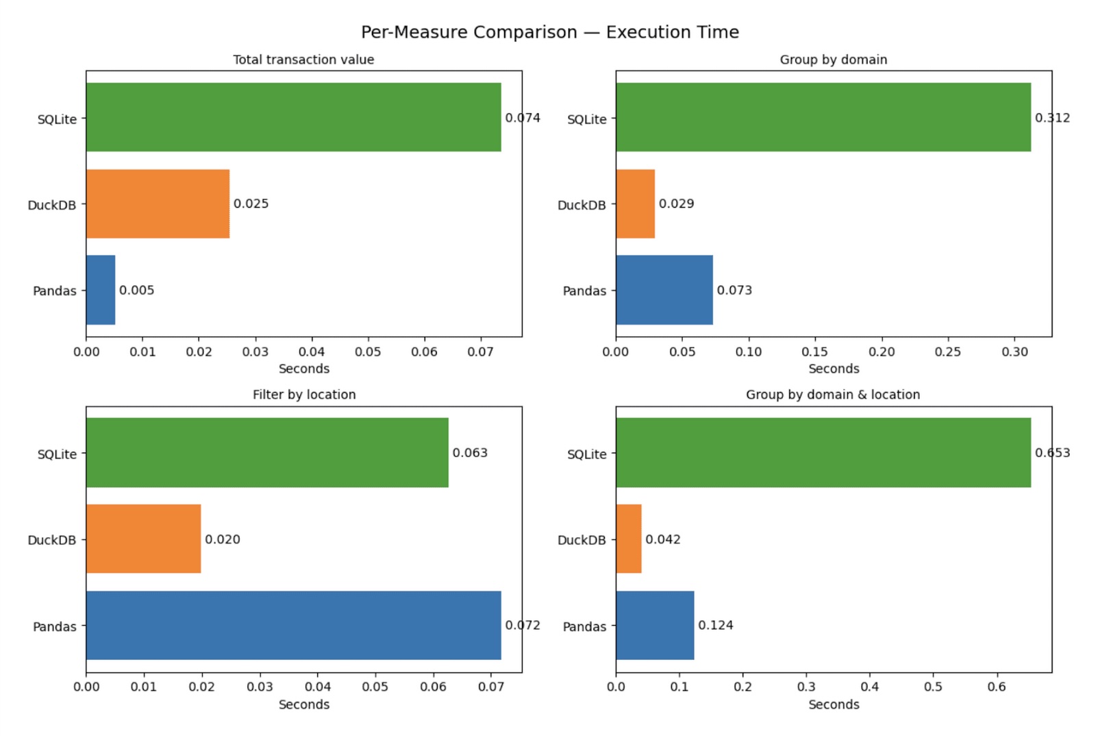
The overall analysis highlighted:
- DuckDB: Consistently fastest or near-fastest with moderate memory usage, making it the most balanced choice.
- Pandas: Showed extreme variance, being the fastest/most efficient for the simplest aggregation but one of the slowest/heaviest for more complex grouping.
- SQLite: Generally the slowest across the board.
My Take
- Data Loading: Pandas’
read_excelis the go‑to for quick prototyping, but it can be memory‑heavy for 1 M+ rows. - DuckDB: Designed for analytical workloads, it leverages in‑memory columnar storage, giving a sweet spot between speed and RAM usage.
- SQLite: Lightweight and file‑based, it’s handy for small‑scale analytics but can lag when heavy joins or aggregations are involved.
From a tech lens, the benchmark underscores that choosing the right engine hinges on your workload: raw speed vs. memory efficiency vs. deployment simplicity. Keep the dataset size, query complexity, and resource constraints in mind, and you’ll pick the engine that turns data into insight faster.
Key Takeaway: “Speed matters, but so does context. Match your tool to the task, and your data will thank you.”
Bulk Load Showdown: Static vs Dynamic
The article contrasts two critical methods for importing multi-file CSV datasets into a SQL Server table using the BULK INSERT statement: Static and Dynamic bulk inserts. The static approach is straightforward, requiring each source file’s name to be explicitly coded in the T-SQL script. It’s perfect for scenarios where the file names remain constant across successive import jobs, though the file content can and will change. The provided example demonstrates a five-part T-SQL solution that uses staging tables for three fixed-name CSV files (IWM, DIA, SPY), loads them one by one, and inserts the data with a ticker prefix into a final, consolidated table named dbo.ticker_date_price. This method is easier to learn and ideal for initial development or fixed data pipelines.
In contrast, the dynamic approach uses a control table (a temp table, #ticker_files, in the example) to store file paths and associated metadata, like the ticker. A WHILE loop then iterates through this control table, constructing and executing a BULK INSERT statement using dynamic SQL for each file. This design is highly flexible, as the list of files to be loaded can change between runs simply by altering the content of the control table. The dynamic script uses a reusable temporary staging table (#staging_price_data) to handle each file’s data before inserting it into the permanent dbo.ticker_date_price table. The article concludes by demonstrating a simple financial analysis—calculating the overall percentage price change—that can be performed on the consolidated table, highlighting the value of an efficient import process.
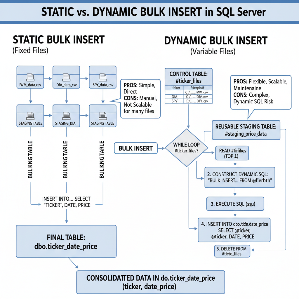
Static Solution Code Highlights
The static solution manually scripts out the load for each of the three files, relying on fixed file names and dedicated staging tables for each import.
Part 1: Target Table Setup
-- Part 1
use [T-SQLDemos];
-- Conditionally drops existing table/constraint
if object_id('dbo.ticker_date_price', 'U') is not null
BEGIN
    -- ... drop constraint and table logic ...
    drop table dbo.ticker_date_price;
END
create table dbo.ticker_date_price (
   ticker nvarchar(10),
   date date,
   price decimal(10,2)
   constraint pk_ticker_date PRIMARY KEY (ticker, date));
- This section sets the stage by selecting the database and ensuring the final destination table, dbo.ticker_date_price, is clean for a fresh run. Crucially, it defines a Primary Key on (ticker, date), enforcing data integrity and uniqueness for the combined data.
Part 2, 3, & 4: Staging and Transformation (The Key Transformation)
-- Part 2 (Similar code structure for Parts 3 & 4)
-- ... drop and create staging table (e.g., dbo.IWM_1993_1_22_2025_7_31)
create table dbo.IWM_1993_1_22_2025_7_31 (
   date date,
   price decimal(10,2));

-- Bulk Insert: Loads data from a fixed path/file into the staging table
bulk insert dbo.IWM_1993_1_22_2025_7_31
from 'C:\CSVsForSQLServer\IWM_1993_1_22_2025_7_31.csv'
with (
    firstrow = 2, -- Skips header row
    fieldterminator = ',',
    rowterminator = '\n',
    tablock);

-- Transformation: Inserts data from staging table into final table, adding the Ticker
insert into dbo.ticker_date_price
select 'IWM' ticker, date, price from dbo.IWM_1993_1_22_2025_7_31
- Explanation: This block, repeated for each ticker (IWM, DIA, SPY), defines a temporary staging table, executes the BULK INSERT using the hardcoded file path, and then performs the critical data transformation: appending a static ticker value (e.g., ‘IWM’) to the date and price columns before inserting the rows into the final consolidated table.
Dynamic Solution Code Highlights
The dynamic solution uses control structures to iterate over files, making it flexible for changing source lists.
Part 1 & 3: Control Table and Reusable Staging Table
-- Part 1: Create a temp control table to hold tickers and file paths
if object_id('tempdb..#ticker_files') is not null drop table #ticker_files;
create table #ticker_files (
    ticker nvarchar(10),
    filepath nvarchar(255));
insert into #ticker_files (ticker, filepath) values
    ('IWM', 'C:\CSVsForSQLServer\IWM_1993_1_22_2025_7_31.csv'),
    ('DIA', 'C:\CSVsForSQLServer\DIA_1993_1_22_2025_7_31.csv'),
    ('SPY', 'C:\CSVsForSQLServer\SPY_1993_1_22_2025_7_31.csv');

-- Part 3: Create a reusable staging table
if object_id('tempdb..#staging_price_data') is not null drop table #staging_price_data;
create table #staging_price_data (
    date date,
    price decimal(10,2));
- Explanation: The #ticker_files table is the control table, the centerpiece of the dynamic process. It lists all files to be imported. #staging_price_data is a temporary table that is reused for every file in the loop, unlike the static solution’s three separate staging tables.
Part 4: The Dynamic Execution Loop (The Key Transformation)
-- Part 4: Loop through control table
declare @ticker nvarchar(10), @file nvarchar(255), @sql nvarchar(max);
while exists (select 1 from #ticker_files)
begin
    select top 1 @ticker = ticker, @file = filepath from #ticker_files;

    truncate table #staging_price_data; -- Important: clear staging table for the next file

    -- Construct Dynamic SQL String
    set @sql = '
    bulk insert #staging_price_data
    from ''' + @file + '''
    with (
        firstrow = 2,
        fieldterminator = '','',
        rowterminator = ''\n'',
        tablock
    );';

    exec(@sql); -- Execute the BULK INSERT command

    -- Transformation: Inserts data from staging table, adding the Ticker from the variable
    insert into dbo.ticker_date_price (ticker, date, price)
    select @ticker, date, price from #staging_price_data;

    delete from #ticker_files where ticker = @ticker; -- Removes processed file from control table
end
- Explanation: This WHILE loop drives the whole process. It fetches the next file path and ticker into variables (@file and @ticker). The key feature is the construction and execution of the dynamic SQL string (@sql) which parameterizes the file path for the BULK INSERT command. The critical transformation here is that the @ticker variable—sourced from the control table—is used in the subsequent INSERT INTO statement, ensuring the correct financial identifier is appended to the data from the currently loaded file. The loop terminates when the control table is empty.
My Take
This is a classic architectural trade-off that every data engineer faces: rigidity versus flexibility. The article cleanly lays out the two primary patterns for ETL operations involving multiple source files. For a beginner or a fixed-scope project with only a few files that never change names, the Static approach is the clear winner. Its simplicity means less debugging, easier code review, and virtually zero risk of SQL injection (a key consideration whenever dynamic SQL is used).
However, my professional opinion leans heavily toward the Dynamic solution for any production environment intended to scale or adapt. Manual coding of file names is a maintenance bottleneck and an anti-pattern for scalability. The dynamic approach, by leveraging a file control table, decouples the logic from the data source list. This is a robust design pattern—you simply update the control table, and the import process naturally handles the new or changed files. The use of dynamic SQL (EXEC(@sql)) combined with a WHILE loop is the right way to achieve this file-by-file processing in T-SQL, though developers should always be meticulous about parameterization to prevent security issues. The article is spot-on: for an increasing number of source files, the dynamic method’s initial complexity is quickly overshadowed by its superior flexibility and ease of maintenance.
Final Thoughts
My key takeaway from this dual exploration is clear: Context is the supreme king in data engineering. We can’t afford to be tool-agnostic or method-agnostic. The DuckDB benchmark proves that a tool designed for analytical workloads (like columnar storage) will outperform general-purpose tools (like SQLite or Pandas for complex groupings) when querying large data, underscoring the importance of matching the engine to the query task. Simultaneously, the BULK INSERT showdown confirms that an initial investment in architectural flexibility—like the control table and dynamic SQL pattern—pays exponential dividends in maintenance and scalability for ETL tasks. A static, hardcoded import process (Static BULK INSERT) is a time bomb in a production environment. The truly efficient data platform must integrate both lessons: use specialized, high-performance tools for analysis, and build flexible, dynamic frameworks for data ingestion. Don’t just chase raw speed; chase the sustainable, scalable architecture. The dynamic BULK INSERT is precisely that—an architecture that lets your data grow without forcing you to rewrite your code constantly.